
Yes, a Poisson goal model can produce defensible scoreline probabilities. Estimate each team's expected goals, often written as lambda (λ), then run those numbers through a scoreline matrix to price the common markets: 1X2, Over/Under, and Both Teams to Score (BTTS).
The one-line recipe: combine attack strength, defense strength, and the league's scoring baseline to get a team's λ for a given fixture, feed that λ into the Poisson probability mass function, multiply the two teams' distributions together to build a score grid, then sum the right cells to get your market probabilities.
Here's the compact version you can act on immediately, before we get into the mechanics:
- Pull at least one full season of match-level goal data for the league you're modeling.
- Calculate each team's attack rating (goals scored relative to league average) and defense rating (goals conceded relative to league average).
- Multiply attack, defense, and league baseline (plus a home-advantage adjustment) to get λ for each side in a fixture.
- Run both lambdas through the Poisson formula to get a probability for every scoreline from 0-0 up to your cap (usually 6-6 or higher).
- Sum the matrix cells to get 1X2, Over/Under, and BTTS probabilities, then compare those to market odds to check for value.
- Expect the raw model to slightly underprice 0-0 and 1-1 draws until you apply the Dixon-Coles correction covered later in this guide.
Key Takeaways
A Poisson goal model turns per-team expected goals into a scoreline matrix, and that matrix, corrected for low-score dependence, is the foundation for pricing 1X2, Over/Under, and BTTS markets accurately.
| Point | Details |
|---|---|
| Anchor lambdas to baselines | Compute attack and defense ratings relative to league averages, then multiply by home advantage to get fixture-specific λ. |
| Build the matrix correctly | Multiply two independent Poisson pmfs to form the scoreline grid, then sum the right cells for each market. |
| Fix known weak spots | Apply Dixon-Coles for low-score accuracy and Negative Binomial or hierarchical pooling when overdispersion or small samples show up. |
| Validate before trusting output | Use walk-forward testing, calibration plots, and Brier score to confirm your probabilities match observed outcomes. |
| Check the market, not just the model | Normalize market odds for bookmaker vig before comparing them against your model's probabilities to spot real value. |
| Consider a ready-made overlay | Lottooracleapp offers a curated sports-prediction overlay for readers who want quick insights without building a Poisson pipeline themselves. |
Where to Go Deeper on Poisson Goal Modeling
Maher's original 1982 framework still underpins the double Poisson regression approach used in most modern implementations, and it's worth reading if you want the academic grounding behind attack, defense, and home-advantage coefficients. For a code-first walkthrough, the step-by-step Python build covers the same strengths-and-baseline recipe used in this guide, including the Dixon-Coles correction in more mathematical detail.
If you want to see the regression case study worked through with actual probability-to-odds conversion, the sports-betting-textbook case study is a solid next stop. And for a grounded comparison of Poisson against machine learning alternatives, the arXiv analysis across five European leagues is the clearest evidence available that model choice matters less than most tutorials suggest.
Anyone building models for leagues with limited historical data should also read the hierarchical Bayesian comparison thesis before deciding whether partial pooling is worth the added complexity for their specific use case.
Table of Contents
- What Is a Poisson Goal Model and Why Does It Work for Football?
- How Do You Build a Basic Poisson Goals Model?
- What Does a Worked Poisson Example Look Like?
- How Do You Turn Model Probabilities Into Betting Value?
- Where Does the Poisson Model Break, and What Fixes That?
- How Do You Validate a Poisson Model Before Trusting It?
- What Data and Engineering Practices Actually Matter?
- Sources
What Is a Poisson Goal Model and Why Does It Work for Football?
A Poisson distribution describes the probability of a certain number of events happening in a fixed window, when those events occur independently and at a roughly constant average rate. For football, the "events" are goals, the "window" is 90 minutes, and the constant rate is λ, the expected number of goals a team will score against a given opponent.
The formula looks intimidating on paper but is simple in practice:
P(X = k) = (λ^k × e^(−λ)) / k!
Here, k is the number of goals you're calculating the probability for, and λ is the expected goals for that team in that match. Plug in λ = 1.4 and k = 2, and you get the probability that team scores exactly two goals.
Three assumptions make this work, and it's worth knowing exactly what you're accepting when you use them:
- Independence. Each goal is assumed to happen without influencing the next one. In reality, a team leading 3-0 often eases off, which breaks this assumption slightly.
- Constant rate. The scoring rate is treated as fixed for the full 90 minutes, even though most teams create more danger in certain stretches (the last 15 minutes, for instance) than others.
- Equidispersion. The variance of goals scored should equal the mean. Real football data often violates this, which is the model's most common weak spot.
Football goals fit the Poisson shape well enough to be useful, even though they don't fit perfectly. Maher's 1982 paper established the double Poisson regression approach still used today, modeling each team's goals as a separate Poisson process shaped by attack strength, defense weakness, and home advantage. Later empirical checks have found that real match data tends to show slightly more variance than a pure Poisson predicts, meaning you see more 0-0 draws and more high-scoring blowouts than the textbook distribution alone would suggest. That gap is small enough that Poisson remains a solid starting point, but large enough that you'll want a fix, which we cover later.
Quick stat check: in a tournament sample of 64 matches, researchers found a variance-to-mean ratio greater than one for goals scored, a textbook sign of overdispersion. That single number explains most of the calibration complaints you'll read about naive Poisson models online.
How Do You Build a Basic Poisson Goals Model?
Building a working model is a sequence of concrete steps, not a single calculation. Here's the order that actually produces usable numbers.
- Collect match data. Pull final scores, home/away designation, and date for every match in your target league, ideally covering at least one full season (38 matches per team in a standard European top flight) so your sample size supports stable estimates.
- Clean the data. Remove abandoned or voided matches, standardize team names across seasons (promoted and relegated clubs cause the most headaches here), and flag any matches with unusual circumstances (behind-closed-doors games, for instance).
- Calculate league baselines. Find the average goals scored per home team and per away team across the whole league. These two numbers anchor everything that follows.
- Calculate attack and defense ratings. For each team, divide their average goals scored by the league average (that's attack strength), and divide their average goals conceded by the league average (that's defense weakness, since a higher number means a leakier defense).
- Fold in home advantage. Home teams typically score more and concede less than the same team would on the road, so apply a home multiplier separately from the attack/defense ratings, or let a regression model estimate it directly.
- Compute fixture lambdas. For a specific match, multiply the home team's attack rating, the away team's defense rating, the league's home-scoring baseline, and the home advantage factor together to get the home team's λ. Reverse the roles for the away team's λ.
There's a more rigorous version of steps 3 through 6 that most serious modelers eventually adopt: a log-linear Poisson regression. Instead of computing simple ratios, you fit a model where log(λ) equals the sum of an attack coefficient, a defense coefficient, and a home-advantage coefficient, estimated jointly across every team and match in your dataset. This is exactly the double Poisson regression structure that has anchored academic football modeling since Maher's original work, and it handles teams with uneven schedules far better than manual ratios do.
| Approach | Best for | Tradeoff |
|---|---|---|
| Simple attack/defense ratios | Quick analysis, small datasets, transparency | Sensitive to small samples and schedule imbalance |
| Log-linear Poisson regression | Full-season modeling with consistent data | Requires a GLM library and more setup |
| Hierarchical/Bayesian pooling | Leagues with promoted teams or thin data | Slower to fit, but stabilizes weak signals |
Pro Tip: Start with simple ratios to sanity-check your data pipeline, then move to Poisson regression once you trust the inputs. Debugging a regression on bad data wastes more time than debugging bad data with simple math first.
What Does a Worked Poisson Example Look Like?
Toy numbers make the mechanics click faster than any formula alone. Assume a fictional league where the average home team scores 1.5 goals and the average away team scores 1.1 goals per match.
| Team | Attack rating | Defense rating | Role in this fixture |
|---|---|---|---|
| Home United | 1.30 | 0.90 | Home |
| Away City | 0.85 | 1.20 | Away |
To compute Home United's λ: multiply their attack rating (1.30) by Away City's defense rating (1.20) by the league's home baseline (1.5). That gives you roughly 2.34 expected goals. For Away City's λ: multiply their attack rating (0.85) by Home United's defense rating (0.90) by the league's away baseline (1.1), landing near 0.84 expected goals.
The pseudocode for turning those two lambdas into a full scoreline grid looks like this:
home_lambda = home_attack * away_defense * league_home_avg
away_lambda = away_attack * home_defense * league_away_avg

for i in range(0, max_goals):
    for j in range(0, max_goals):
        home_prob = poisson_pmf(i, home_lambda)
        away_prob = poisson_pmf(j, away_lambda)
        matrix[i][j] = home_prob * away_prob
Running that loop with home_lambda near 2.34 and away_lambda near 0.84 produces a grid where the most likely single scoreline is 2-1 to the home side, with 2-0 close behind. To read the matrix for market probabilities:
- Sum every cell where the home team's goal count exceeds the away team's for the home win probability.
- Sum the diagonal (0-0, 1-1, 2-2, and so on) for the draw probability.
- Sum every cell where away goals exceed home goals for the away win probability.
- Sum all cells where total goals equal 3 or more for an Over 2.5 goals probability.
This exact outer-product method, attack times defense times baseline feeding into two independent Poisson pmfs, is the standard recipe used across most public Poisson goal model tutorials, and it's worth building once by hand before you automate it, so you understand exactly what each cell in the matrix represents.
How Do You Turn Model Probabilities Into Betting Value?
Converting a probability into implied decimal odds is a one-step calculation: divide 1 by the probability. If your model says Home United has a 52% chance to win, the fair decimal odds are 1 divided by 0.52, or about 1.92.
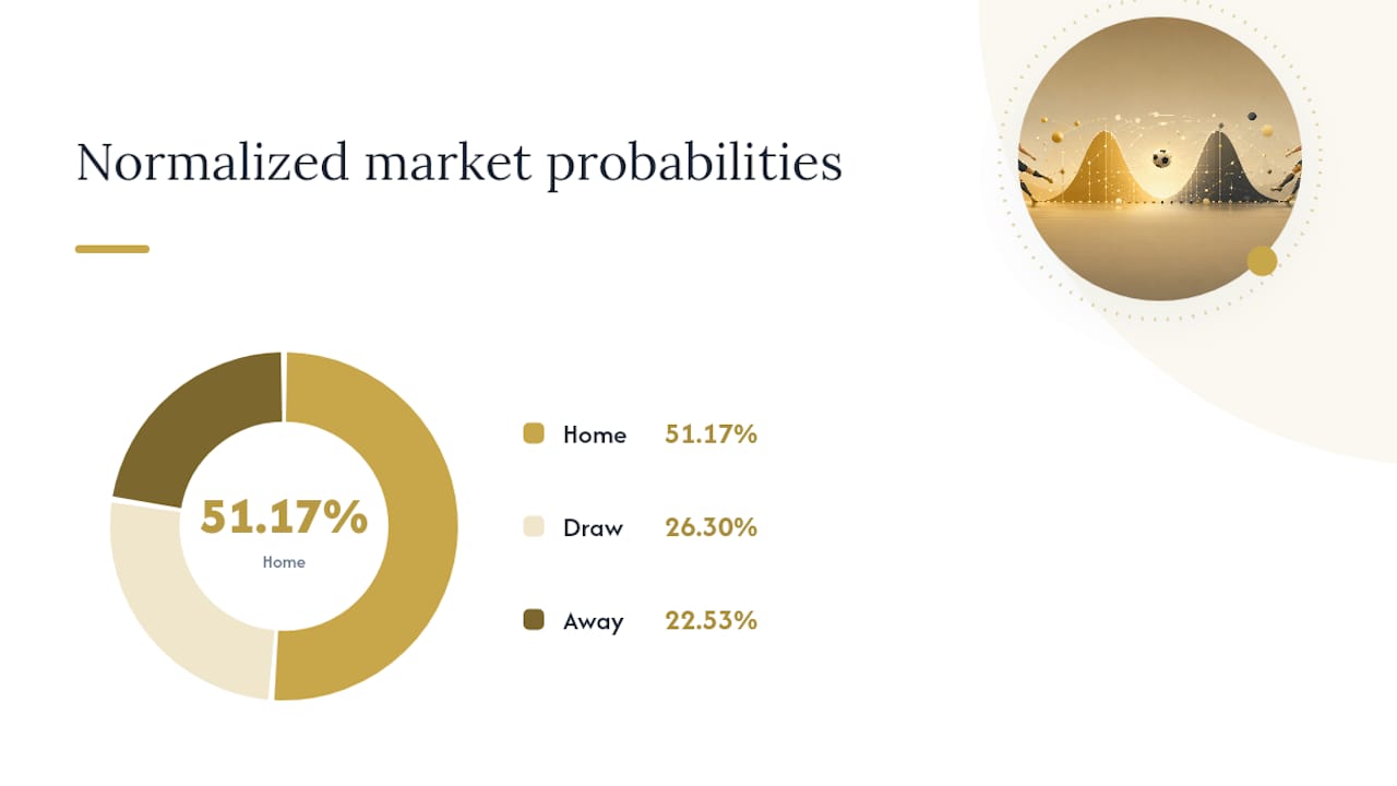
Bookmakers never offer fair odds, though. They build in a margin (often called the vig or overround) by shading every outcome's odds slightly against the bettor. A market showing 1.85 / 3.60 / 4.20 for home/draw/away will sum to more than 100% in implied probability once you convert each price back with 1/odds. That excess is the bookmaker's edge, and you need to strip it out before comparing your model's numbers to the market's.
A simple vig-normalization example: if your three implied probabilities from the market sum to 106%, divide each individual probability by 1.06 to rescale them back to 100%. Now you have the market's true estimate of each outcome, stripped of margin, ready to compare directly against your model's output.
- Compute 1X2 probabilities directly from your scoreline matrix, as shown in the previous section.
- Aggregate every cell with total goals of 3 or higher for Over 2.5, and every cell where both home and away goals are at least 1 for BTTS Yes.
- Compare your model's probability for each outcome against the vig-normalized market probability for the same outcome.
- Flag a potential value bet when your model's probability exceeds the market's normalized probability by a meaningful margin, many analysts use something in the range of 3 to 5 percentage points as a rough threshold before committing real stakes.
- Size any stake conservatively relative to your bankroll rather than betting flat amounts regardless of edge size.
Quick stat check: research comparing Poisson-based approaches against several machine learning models across five European top leagues found comparable performance for total-goals prediction, with feature engineering and data quality mattering more than which specific model architecture you pick. That's a useful reality check before you spend weeks tuning a neural network instead of cleaning your input data.
Where Does the Poisson Model Break, and What Fixes That?
The single biggest practical failure of a plain Poisson model is overdispersion: real-world variance in goals scored tends to run higher than the mean, while a pure Poisson process assumes they're equal. That mismatch shows up as too few predicted 0-0 and 1-1 draws and too few predicted blowouts, because the naive model compresses the tails of the distribution toward the average.
A second structural issue: the model assumes each team's goals are independent of the other team's goals within the same match. In practice, low-scoring games have a subtle correlation, a 0-0 is slightly more likely than independence alone would predict, because both teams are often playing cautiously for the same tactical reasons.
The Dixon-Coles correction targets exactly this problem. It applies a small multiplicative adjustment to the 0-0, 1-0, 0-1, and 1-1 cells of the scoreline matrix, nudging the model's low-score predictions closer to what actually happens on the field, and it pairs that fix with a time-weighting scheme that gives recent matches more influence than older ones when estimating team strengths.
That single, targeted tweak, documented in detail by Build a Poisson Goals Model in Python, is often enough to close most of the gap between a naive Poisson and a well-calibrated one.
Beyond Dixon-Coles, three other standard fixes address different symptoms:
- Negative Binomial regression adds a dispersion parameter that lets variance exceed the mean, directly addressing overdispersion rather than patching individual cells.
- Bayesian hierarchical models apply partial pooling across teams, which stabilizes ratings for clubs with limited match history, newly promoted teams being the clearest example, by borrowing strength from the league-wide pattern.
- Time-weighting discounts older matches on a decay curve so a team's rating reflects current form rather than treating a match from ten months ago the same as last weekend's result.
Pro Tip: If you only have budget to implement one fix, start with Dixon-Coles. It's a small correction with an outsized effect on draw and low-score accuracy, which is exactly where naive Poisson models lose the most credibility.
Hierarchical Bayesian approaches deserve a specific mention for anyone modeling a league with irregular data, lower divisions, cup competitions, or leagues with frequent promotion and relegation. Comparative research on Poisson GLMs versus Bayesian hierarchical models found that partial pooling reduces bias specifically when the model is misspecified or when certain teams have too few matches for a stable standalone estimate.

How Do You Validate a Poisson Model Before Trusting It?
A model that looks reasonable on paper can still be badly miscalibrated, so validation isn't optional if you plan to use the output for real decisions. Follow this sequence before you trust any output:
- Split your data chronologically. Train on one stretch of matches and test on a later stretch you haven't touched, never randomly shuffle football data, since that leaks future information into your training set.
- Run walk-forward validation. Refit the model after each round of matches and test only on the next round, rolling forward through the season, to simulate how the model would have performed in real time.
- Check your sample size. A handful of matches per team produces unstable attack and defense ratings, most practitioners want at least half a season, and ideally a full season or more, before trusting team-specific parameters.
- Plot a calibration curve. Bucket your predicted probabilities (0-10%, 10-20%, and so on) and check whether the actual outcome frequency in each bucket matches the predicted range.
- Calculate the Brier score. This is the mean squared difference between predicted probability and actual outcome (scored as 0 or 1), lower is better, and it's the standard scoring rule for comparing probabilistic forecasts against each other.
- Review a confusion matrix for predicted result bands. Group your predictions into confidence bands (say, 40-50%, 50-60%, 60-70% for the favorite) and see whether higher-confidence bands actually win more often.
Two failure signals show up repeatedly when analysts run this process. The first is systematic overconfidence, where your 70% predictions only win 55% of the time, a sign your model's probabilities need shrinking toward the mean.
Quick stat check: applied Poisson regression using goal averages, home advantage, and offensive/defensive strengths achieved fairly strong predictive accuracy when tested against the actual 2017-2018 English Premier League season, evidence that a carefully built basic model can hold up under real backtesting rather than just looking plausible in a spreadsheet.
What Data and Engineering Practices Actually Matter?
Data quality determines your ceiling more than model sophistication does. Public sources like league APIs, open match-result feeds, and providers such as StatsBomb give you the raw goal, date, and venue data you need, but every source has gaps, postponed fixtures, replayed matches, and inconsistent team naming across seasons being the most common headaches.
Handle missing or inconsistent results by excluding rather than guessing. A match with a disputed final score or an abandonment shouldn't be imputed with an average value, it should simply be dropped from the training set, since a fabricated data point does more damage than a smaller sample size.
A few engineering details separate a functional model from a fragile one:
- Cap your max_goal value in the scoreline matrix at something reasonable, 8 or 10 goals per side is plenty, since probabilities beyond that range round to effectively zero and just waste computation.
- Apply shrinkage for newly promoted teams. A club with no top-flight history has no reliable attack/defense rating yet, so blend their early-season estimate toward the league average until enough matches accumulate.
- Use vectorized matrix operations rather than nested loops when computing the scoreline grid across many fixtures at once, this matters once you're scoring an entire matchday rather than a single fixture.
- Time-weight your training window. A simple exponential decay on match age, giving matches from three months ago more weight than matches from a year ago, captures current form without discarding your full dataset.
Open-source tooling can save you from reinventing this pipeline. Packages like the goalmodel R library already implement Poisson, Negative Binomial, and Dixon-Coles variants with configurable weighting, which is a reasonable starting point if you'd rather adapt existing code than write a GLM fitter from scratch.
Pro Tip: Watch your variance-to-mean ratio on each team's scored and conceded goals before you commit to a model family. A ratio close to 1.0 means plain Poisson is fine; anything meaningfully above 1.0 is your signal to switch to Negative Binomial or add hierarchical pooling. For readers who also apply probabilistic thinking to other games of chance, the fundamentals covered in lottery probability basics walk through similar expected-value logic in a simpler setting.
When Is a Poisson Baseline the Right Call?
The honest answer is that a well-built Poisson model, with Dixon-Coles and sensible time-weighting layered on, gets you most of the way to a production-quality forecast without the overhead of a machine learning pipeline. Comparative research backs this up directly: Poisson approaches hold their own against several ML models for total-goals prediction, and the gap between them often comes down to feature quality rather than model architecture.
Where I'd escalate past a basic Poisson: leagues with thin historical data, competitions with heavy promotion and relegation churn, or any situation where you need the model to explain itself to a non-technical audience. A hierarchical Bayesian model handles small samples better, but a simple attack/defense Poisson model is far easier to audit line by line when something looks wrong. For anyone weighing whether to build a custom pipeline or lean on a broader comparison of statistical versus algorithmic approaches, a resource like the practitioner's guide on football prediction algorithms is a useful second opinion before you commit engineering time.
Deployability matters more than most tutorials admit. A model you can explain in one paragraph, and re-fit in under a minute when new results come in, beats a marginally more accurate model that takes a data scientist to debug when it misfires on a Tuesday afternoon.
Building your own vs. using a ready-made overlay
Building a Poisson pipeline from scratch gives you full control over your assumptions, your data sources, and every parameter in the model, and that transparency is exactly why analysts and serious bettors favor the DIY route. It takes real time, though: sourcing clean data, fitting and validating a regression, and maintaining the pipeline as each new matchday's results come in.

If you'd rather skip the spreadsheet work and still get a curated view of upcoming matchups, Lottooracleapp's sports matchup predictions fold pattern analysis and historical trends into a straightforward daily readout, no regression fitting required on your end. That's a genuinely different tool for a genuinely different reader: the DIY Poisson route suits someone who wants to audit every coefficient themselves, while a subscription overlay suits someone who wants a fast, curated signal without building the machinery behind it.
Lottooracleapp is built as an entertainment-oriented prediction and insights platform, not a betting service, and it doesn't sell tickets or place wagers on your behalf. If you're curious what a ready-made overlay looks like alongside your own model's output, you can check the Lotto Oracle platform and compare its sports predictions against your own scoreline matrix for a given weekend. Play responsibly, and treat any prediction tool, statistical or otherwise, as one input among several rather than a guarantee.
Sources
- PMC article on double Poisson regression and football match modelling
- Match predictions in soccer: Machine learning vs. Poisson approaches (arXiv / DOI)
- Build a Poisson Goals Model in Python — SoccerAnalytics
- Predicting Final Result of Football Match Using Poisson Regression Model - IOPscience